10. Embedded Atom Method (EAM) Simulations with MedeA
This application note shows the use of the embedded atom method (EAM) with LAMMPS in the MedeA®[1] Environment. It reviews the concept of the method and illustrates its use by computing the density, bulk modulus, vacancy formation energy, and melting of copper.
Keywords: Embedded Atom Method, EAM, LAMMPS, interatomic potentials, forcefields
10.1. Introduction
The Embedded Atom Method (EAM) is an efficient approach for computing structural, thermo-mechanical, and transport properties of metals and alloys. Within the EAM description, the evaluation of energy and forces, even for large assemblies of atoms, is several orders of magnitude faster than comparable first-principles calculations and this performance scales linearly with the number of atoms. Hence EAM calculations are able to span length and time scales beyond those accessible to first-principles methods. This application note provides an overview of the embedded atom method [2], its use within the MedeA Environment, and it illustrates properties obtained with this method.
10.2. Purpose and Concept
The purpose of the embedded atom method (EAM) is the rapid computation of materials properties from models containing thousands to millions of atoms while retaining key characteristics of metallic bonding.
As its name implies, the EAM accounts for the behavior of an atom placed at a point with an electron density defined by the chemical environment. The method therefore captures the essential contributions to bonding in metals, namely the gain in total energy due to delocalization of the conduction electrons, which are typically of s- and p-character, and the localized bonding in transition metals due to d-electrons.
Related to the effective medium theory of Norskov and Lang [3], the embedded atom method (EAM) was developed by Daw and Baskes [4]. This approach expresses the total energy of the system as two additive terms, a pairwise sum of interactions between atoms, and an embedding term depending on the electron density at each atomic site, as shown in Equation (1) below.
\(U_{EAM}\) is the total potential energy of the system, \(i\) and \(j\) indicate the unique pairs of atoms within the \(N\) atoms of the system, \(r_{ij}\) is the distance between atoms, \(i\) and \(j\), \(V(r_{ij})\) is a pairwise potential, and \(F(\rho_i)\) is the embedding function for atom \(i\) which depends on the electron density, \(\rho_i\), experienced by that atom. To evaluate a given atom’s embedding function, one needs to compute the electron density at the position of atom \(i\). This is obtained by a superposition of “atomic densities”, which are described by a density function, \(\varphi_j(r)\), as shown in Equation (2).
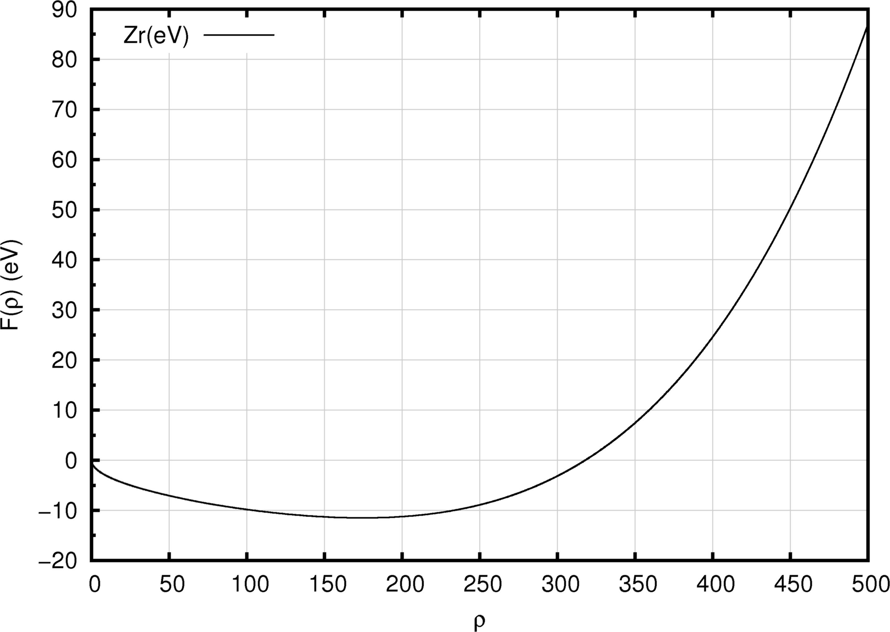
Figure 10.2.1 A typical EAM embedding function, \(F(\rho_i)\), illustrated by the Zr EAM potential of Mendelev and Ackland [5].
The embedding function, \(F(\rho_i)\), provides an essential degree of freedom in the description of metallic bonding. If this term were linear with respect to varying density, the overall energetic description would be equivalent to a standard two body representation. However, the curvature of the embedding term with varying electron density accounts for many-body interactions.
A common form of the embedding function for an EAM forcefield is shown in Figure 10.2.1. Starting at low values, increasing electron density yields progressively more negative embedding energies, until a minimum value is attained beyond which a higher electron density yields less favorable system energies. Figure 10.2.2 and Figure 10.2.3 provide views of the density function, employed to compute the electron density at a given site (Figure 10.2.2), and the pair function (Figure 10.2.3) which is reminiscent of a typical two-body interaction function.
It should be noted that the unit of the density is arbitrary. In the case shown here, the density near the minimum has a value of about 180. This means that if an atom is at a site where the superposition of the density functions from the neighboring atoms is 180, the corresponding embedding energy of that atom is about -11 eV, as can be seen from Figure 10.2.1. Obviously, if the density functions would be 100 times smaller, one can obtain the same embedding energy if also the density in the x-axis of this plot is scaled by the same factor. In fact, the scaling used, for example, by Bonny et al. [6] is indeed about 100 times smaller than that used by Mendelev and Ackland [5]. Thus, mixing EAM forcefields from different sources can be challenging or impractical.
There is a further complication with EAM forcefields, namely a redundancy between the embedding function and the pair function. Bonny et al. [6] overcome this ambiguity by introducing an explicit compensation of the double-counting. While one should be aware of these subtilties, they are of no concern when using forcefields from the comprehensive library available in the MedeA Environment, provided that the selected forcefield is appropriate for the application at hand.
Computing energies and forces based on Equation (1) and (2) is fast as each of the terms are functions of interatomic separation and such separations and their derivatives with respect to atomic coordinates can be rapidly evaluated. In practice, to avoid restricting the form of the functions employed, and to promote computational efficiency, numerically splined look-up tables are used in most EAM calculations for the necessary functions. The resulting EAM files are therefore large numerical tables. For individual elements three such tables are required, representing the pair function, the embedding function, and the density function.
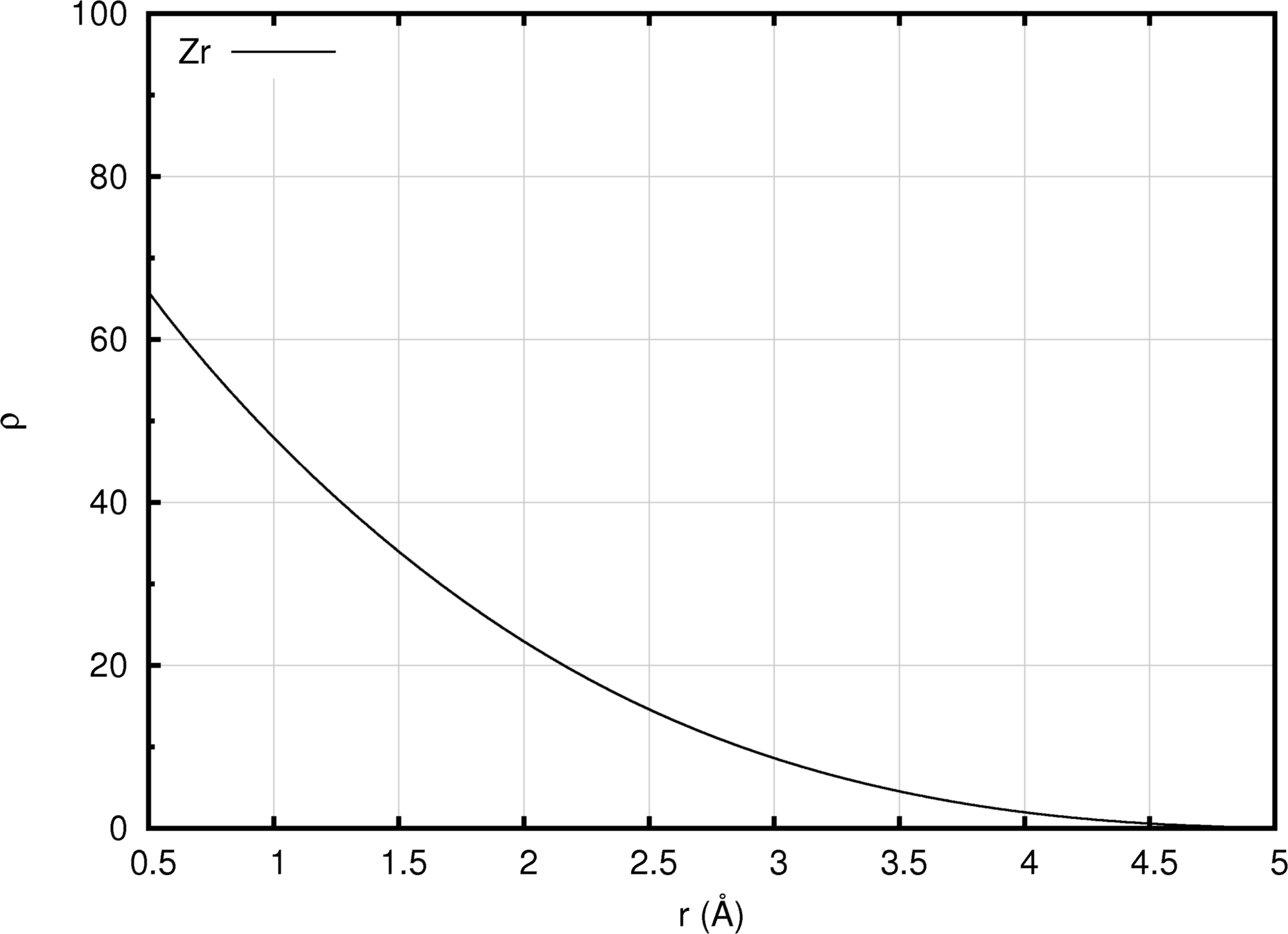
Figure 10.2.2 An EAM density function (illustrated using the Zr EAM forcefield of Mendelev and Ackland [5]).
Handling alloy systems requires provision for functions describing the pairwise interaction of each element, in addition to embedding, and density functions. For an n-component alloy there will be n(n+1)/2 pairwise interaction functions, n-embedding functions, and, associated density functions. The determination of these functions is challenging, and is complicated by the fact that the creation of a description suitable for a single element provides little information for the behavior of that element in an alloy or compound. Consequently, EAM forcefields are typically developed for specific systems and the description of a given element cannot trivially be combined directly with the description for another element, as assumptions about the two density functions, for example, may not be compatible.
The highly specific nature of EAM forcefields is emphasized by examples such as Mendelev and Ackland’s forcefield derivation work for metallic zirconium [5]. Here one parameterization is recommended for the exploration of phase stability and another distinct parameterization for the investigation of defects in the hexagonally close packed (hcp) form of hcp-Zr.
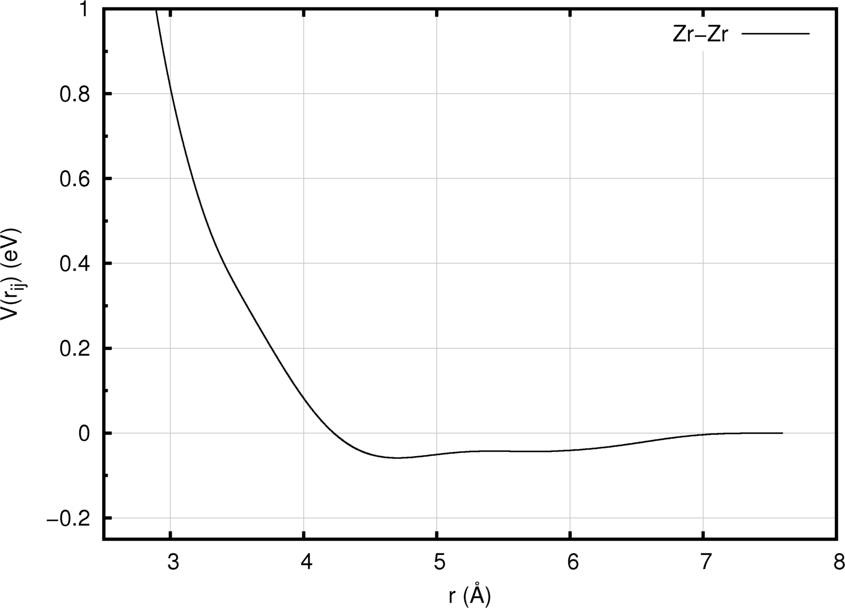
Figure 10.2.3 An EAM pairwise interaction function (Illustrated using the Zr EAM forcefield of Mendelev and Ackland [5]).
Despite such specificity, the merit of EAM forcefields is their ability to rapidly and accurately describe the bonding of metallic systems, provided that the parameters are carefully tuned. EAM forcefields allow the simulation of:
- Structures - for example atomic configurations in the vicinity of vacancies, self-interstitial atoms, grain boundaries, and dislocations
- Energies - for example stacking fault energies and the relative stability of face-centered cubic vs. body-centered cubic phases
- Diffusivity - for example through the use of mean squared displacements of sets of atoms in molecular dynamics trajectories
- Thermal expansivity - for example employing constant pressure molecular dynamics simulations as a function of temperature to predict the response of a lattice to a temperature ramp
- Melting of metals and properties of the liquid state such as density, viscosity, and surface tension as function of temperature.
As EAM forcefield calculations are computationally efficient, large scale simulations can be readily undertaken, as illustrated in the following sections.
10.3. EAM Simulations with MedeA
The MedeA Environment supports standard “Finnis-Sinclair” format EAM forcefield files, with extensions to permit detailed referencing of the source of the particular EAM description and atom type assignment. Such a file contains named sections expressing atom types, any atom equivalences, the standard Finnis- Sinclair format EAM function tables, information for partial charge assignment, and template information to assign forcefield atom types based on rules concerning topology and element type. This overall format is the standard employed by all MedeA Environment forcefields.
In addition to standard Finnis-Sinclair EAM forcefields, the MedeA Environment also supports the EAM parameterization described by Zhou and co-workers [7]. Here, mixing rules have been implicitly included in the design of the forcefield, and any combination of the elements: Cu, Ag, Au, Ni, Pd, Pt, Al, Pb, Fe, Mo, Ta, W, Mg, Co, Ti, or Zr may be handled. It is likely that this generality results in diminished accuracy in some circumstances (see for example [8]). However, when the effects of alloy formation are of interest, in the creation of layered metallic structures, for example, this description is highly effective [7].
An EAM forcefield for modeling plasticity in stainless steel has been developed by Bonny et al. [6], which is also available within the MedeA Environment.
An illustrative EAM calculation performed in the MedeA Environment is shown in Figure 10.3.1. Here a supercell containing 4,000 atoms was initially constructed, and molecular dynamics employed to melt the upper half of this model. A sequence of 2 nano-second simulations were then employed to simulate the interface between the solid and liquid as a function of temperature. This task can be conveniently accomplished using a MedeA flowchart interface, which can be configured to carry out the necessary building and simulation tasks automatically for any desired metal or model type.
Figure 10.3.1 shows a typical configuration from the simulation. In this case the copper system was described with the Zhou EAM forcefield [7]. Then for a range of temperatures, the molecular dynamics trajectory was computed from a half crystalline and half molten starting point and the relative extents of the two regions examined at the culmination of the calculation.
The simulations reveal that below 1375 K, the molten region retreats in the dynamics calculations, indicating that the crystalline system is more stable and crystallizes from such a melt. Above 1375 K, however, the molten region grows relative to the crystalline region. We can conclude that in this simple EAM description and simulation regime, the melting temperature of copper is around 1375 K, which compares quite well with the experimental value of 1358 K, and emphasizes the fact that the simple EAM description captures much of the physics of metallic systems such as copper, if the EAM parameters are carefully fitted.
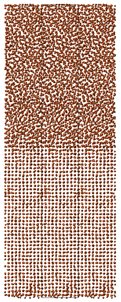
Figure 10.3.1 A copper solid-liquid interface for the molecular dynamics based simulation of melting.
The melting point calculation illustrated by Figure 10.3.1 required around 2 hours of computation time on a modest Linux cluster, demonstrating that such calculations can be rapidly conducted and providing a measure of the types of properties which may be computed. Of course, simulations permit the exploration of a wide range of properties, and are able to address conditions which are difficult to observe directly experimentally, providing a valuable complement to practical investigation. However, one needs to keep in mind the dependence of the results on the training set used in the parameterization of the EAM functions.
The range of properties accessible via EAM calculations is large. Some example properties, obtained using the Zhou [7] copper description are listed in Table 1. In addition to these static properties, as the simulation of melting points illustrates, it is also possible to obtain dynamic properties, such as diffusion coefficients.
| Property | Calculation | Experiment |
|---|---|---|
| Density | 8.85 g/cm3 | 8.94 g/cm3 |
| Vacancy formation energy | 1.28 eV | 1.29 eV [9] |
| Bulk modulus | 133 GPa | 140 GPa |
10.4. Summary
In summary, one of the most important attributes of the EAM is its ability to enable large scale simulations spanning significant time scales while maintaining key aspects of metallic bonding beyond pair-potentials. Thus, it is possible to simulate a wide range of phenomena using this method which are inaccessible to first-principles approaches. The MedeA Environment support for EAM forcefields makes the use of this important simulation method broadly accessible for the first time.
In cases where no appropriate EAM forcefields are available, the MedeA Environment offers the Forcefield Optimizer, a powerful tool for the extension of existing and the creation of new forcefields using MedeA VASP for generating training sets.
Required Modules
- MedeA LAMMPS
- EAM
- MedeA JobServer and TaskServer
| [1] | MedeA and Materials Design are registered trademarks of Materials Design, Inc. |
| [2] | Calculations based on empirical energy functions and parameters derive from early work on vibrational properties of molecular systems, which has led to the term force field or forcefield to describe the functional form and its parameterization. In solid state physics, a classical description of interatomic interactions is often referred to as “interatomic potentials”. In this application note, the terms forcefield and interatomic potential are used interchangeably. |
| [3] | Norskov J. K., Phys. Rev. B 20, 446 (1979); J. K. Norskov and N. D. Lang, Phys. Rev. B 21, 2131 (1980) |
| [4] | Daw M. S. and M. Baskes, Phys. Rev. B 29, 6443 (1984) |
| [5] | (1, 2, 3, 4, 5) Mendelev M. I. and G. J. Ackland, Phil. Mag. Lett. 87, 349 (2007) |
| [6] | (1, 2, 3) Bonny G., D. Terentyev, R. C. Pasianot, S. Ponce, and A. Bakaev, Modelling Simul. Mater. Sci. Eng. 19, 085008 (2011) |
| [7] | (1, 2, 3, 4) Zhou X. W., R. A. Johnson, and H. N. G. Wadley, Phys. Rev. B. 69, 144113 (2004) |
| [8] | Francis M. F., M. N. Neurock, X. W. Zhou, J. J. Quan, H. N. G. Wadley, E. B. Webb III, J. Appl. Phys. 104, 034310 (2008) |
| [9] | Trifthauser W. and J. D. McGervey, Appl. Phys. 6, 177 (1975) |
| download: | pdf |
|---|