26. Self diffusion coefficients for pure acetone and toluene at different temperatures from molecular dynamics simulations
Keywords: Self-diffusion, fluids, viscosity, molecular dynamics
26.1. Introduction
This application note illustrates how to determine self-diffusion coefficients of the pure fluids acetone and toluene using molecular dynamics and the Einstein relation.
Diffusion coefficients are essential parameters in many engineering and industrial processes such as distillation, solvent evaporation, absorption, extraction, multiphase reactions, and many more. Generally, these processes involve several fluid components and phases, varying concentration, and temperature/pressure gradients.
Nuclear Magnetic Resonance (NMR) techniques evaluate self-diffusion coefficients in pure liquids or mixtures. Depending on process conditions (high pressure, high temperature) and compound-inherent hazards, NMR measurements may be challenging and costly. Molecular dynamics simulations have emerged as a viable complement to NMR measurements, and several studies for different liquid mixtures based on common solvents [3] [4] [5] serve as a validation of the computational approach presented below.
Self-diffusion is mass transport in the absence of a chemical concentration gradient, caused by internal kinetic energy (Brownian motion). Self-diffusion coefficients serve as direct input to predictive models for the mole-fraction dependence of mutual-diffusion coefficients [6] [7] [8].
26.2. Molecular Modeling
We use the MedeA simulation environment [1] with the MedeA Diffusion module, the LAMMPS [9] molecular dynamics engine with the PCFF+ forcefield [10] to compute self-diffusion coefficients (D) for pure acetone and pure toluene based on the simplified Einstein diffusion equation:
The numerator is the mean squared displacement (MSD), r is the position, t the elapsed time, d the dimensionality of the simulation cell.
26.2.1. Accuracy and precision
Generally, the accuracy of data computed with classical molecular dynamics depends on the forcefield – here, PCFF+ – used to describe the molecular interactions present in the system. Forcefield parameters for specific molecules and molecular interactions are obtained from experiments or high-precision computational methods. Therefore, when applied within the appropriate application range, they reproduce certain experimental observables very well. In practice, reaching the accuracy attainable by a given forcefield requires precise, well-converged simulations. For self-diffusion coefficients, several parameters control the precision of a calculation:
- The model system size – The number of molecules must be large enough to guarantee good statistical sampling. Thus, for a given fluid density, we need a sufficiently large simulation box [11]. We will discuss this in greater detail in the section on the Finite Size Effect, where we also present methods to evaluate the self-diffusion coefficient in the limit of an infinite-size model.
- The duration of the molecular dynamics simulation – A dynamics run must be long enough for the system to reach the so-called “diffusive regime”, or, in other words, the section of its dynamics trajectory, where the Mean Square Displacement (MSD) increases proportionally with simulation time (t). The time it takes to reach this regime typically increases with the size of the diffusing species and the viscosity of the system. Reaching the diffusive regime may require simulation times ranging from several nanoseconds to hundreds of nanoseconds. The MedeA Diffusion module simplifies and automates the procedure of verifying the transition of the system to the diffusive regime.
- The number of independent initial fluid configurations – For improved statistics, several separate configurations, all of them thermally equilibrated at the same density, should be investigated.
- When dealing with a multicomponent system, precision can also be improved by increasing the number of diffusing species (molecules) in the system; however, care should be taken to avoid the molecules interacting with each other and artificially influencing the apparent diffusivity.
26.2.2. Setting up the simulation
In the MedeA Molecular Builder, we set up individual acetone and toluene molecules and assign them the status of subsets “acetone” and “toluene” before constructing the respective fluid in the MedeA Amorphous Materials Builder. For an initial trial size, we choose a periodic model with a cell length of around 30 \({\mathring{\mathrm{A}}}\).
In Figure 26.2.2.1, we show a workflow to determine diffusion coefficients with the MedeA Diffusion module using LAMMPS as the MD engine. It starts with a Variables stage, by defining input parameters such as temperature, pressure, and the duration for each MD run. First comes a LAMMPS equilibration stage for the density (NVT, NPT), and a step to reset the model cell to this density. This is followed by another LAMMPS stage, which determines the diffusion constant in the microcanonical ensemble (NVE).
In the NVE ensemble, the number of particles, the volume of the cell, and the energy are held constant. Performing the “production” dynamics run in the NVE ensemble ensures that the molecular dynamics trajectories are not altered during the run. Running in the NVT or NPT ensemble, changes to the particle trajectory would occur because of the exchange with the thermostat and barostat, required to keep the temperature and pressure constant.
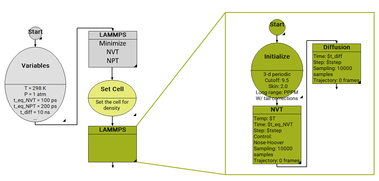
Figure 26.2.2.1 Screenshot of MedeA flowchart for the equilibration of a liquid at given T, P, followed by a diffusion calculation.
26.2.3. Verifying energy and temperature conservation
During the production run, energy and temperature must not show more than a small drift throughout the simulation. Figure 26.2.3.1 shows the running average of the total energy and the temperature during two nanoseconds of NVE simulation with a time step of 1 femtosecond, preceded by thermal equilibration at 328 K for a cell containing 200 toluene molecules.
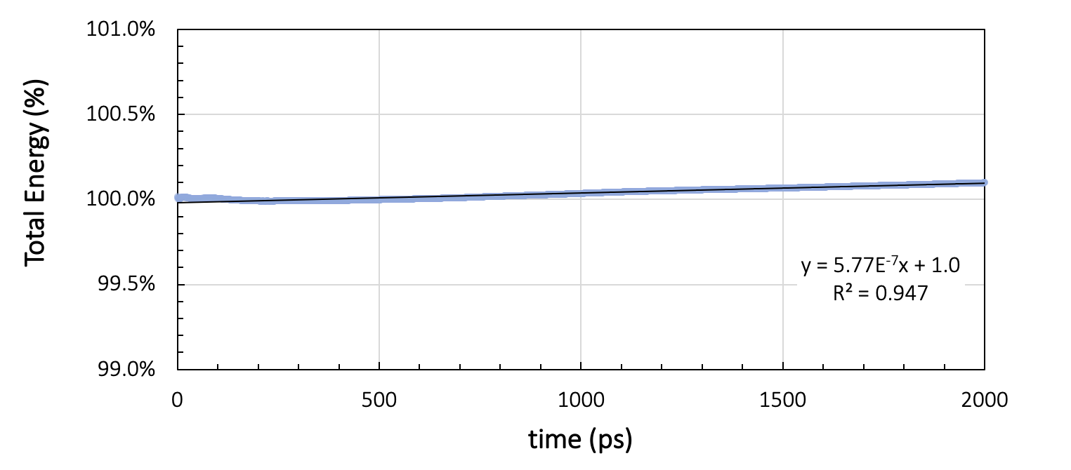
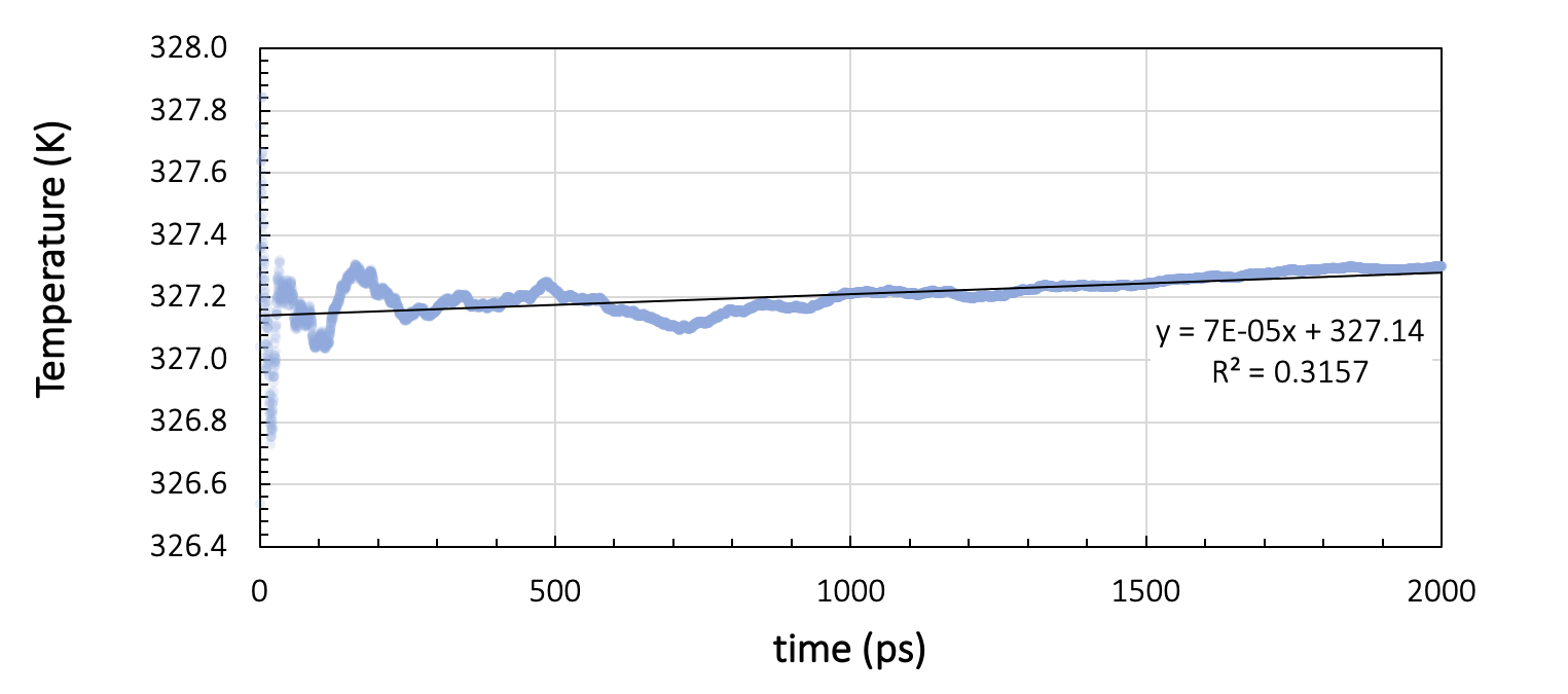
Figure 26.2.3.2 Results for a system of 200 toluene molecules at 328K: Running averages for total energy and temperature during two nanoseconds of NVE simulation.
Ideally, NVE dynamics should conserve the energy, but a slight drift, depending on the integrator, the timestep size, the forcefield, and the temperature, may be observed. In our toluene example in Figure 26.2.3.1, the energy per cell varies by 7.5x10⁻³ kcal/mol over the two nanosecond run. The temperature drift over the same duration is around 0.2 K. Therefore, we can assume the energy to be stable for temperature variations smaller than 0.2 K.
26.2.4. Confirming the diffusive regime
The simulation length must be long enough for the diffusive species to reach the diffusive regime. To confirm this, we check the following parameters:
- The computed slope (m), printed in the MedeA “job.out” file, from a log-log plot of the MSD (Figure 26.2.4.1) averaged over the simulation time for all diffusing species: when the system has reached the diffusive regime, m should be close to 1. In practice, m-values between 0.9 and 1.10 are considered acceptable.
- The square root of the MSD averaged over all diffusing species: it should be comparable to or larger than the simulation box length (L) because only then the diffusing species has sampled a significant part of configuration space. From Figure 26.2.4.2, we conclude that our toluene run with a box length of 30 Ang and the square root of the MSD of ~63 Ang meets this convergence criterion.
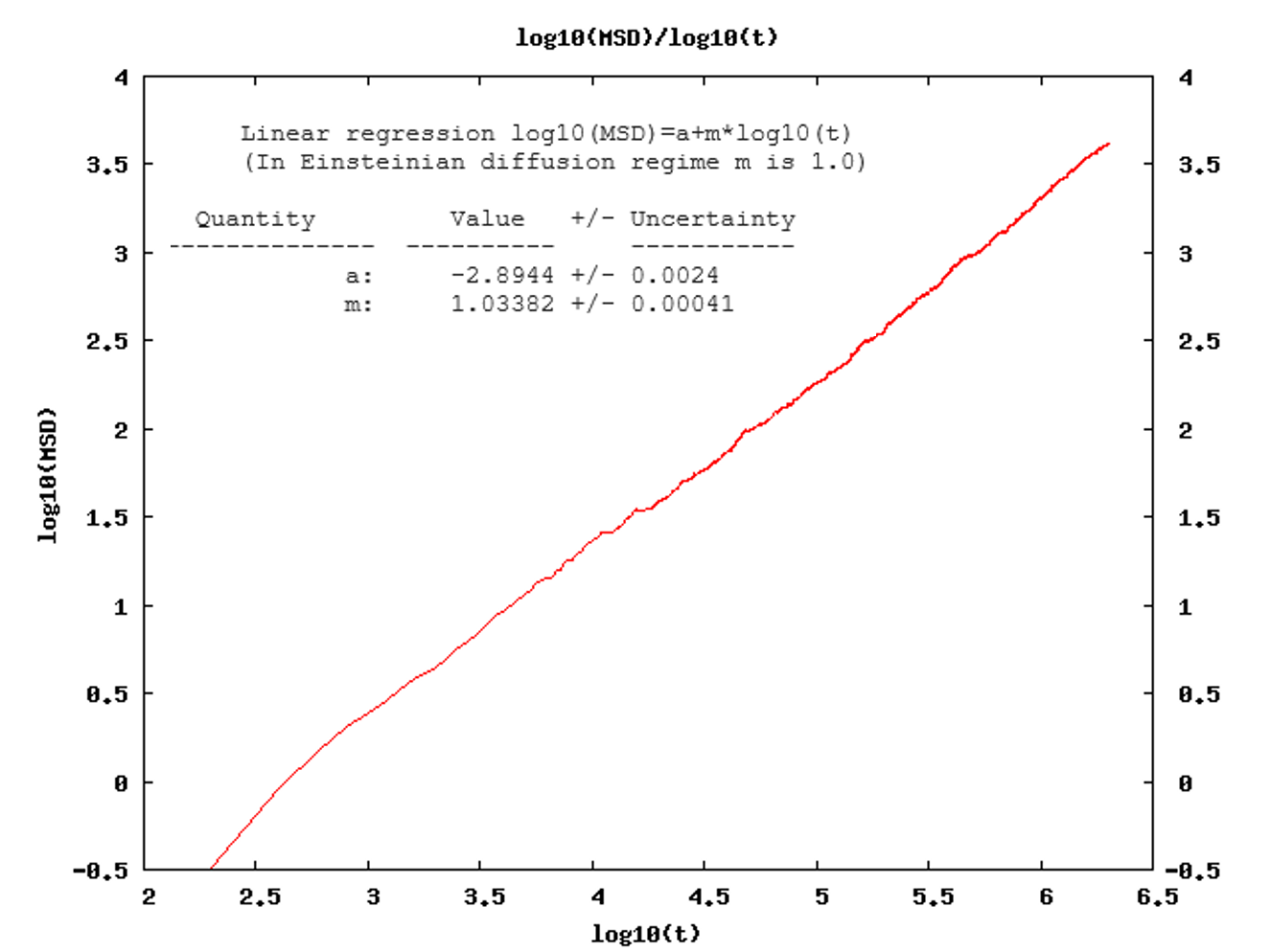
Figure 26.2.4.1 The MedeA Diffusion module plots the log(MSD) versus log(t). The job.out file provides the results of the linear regression.
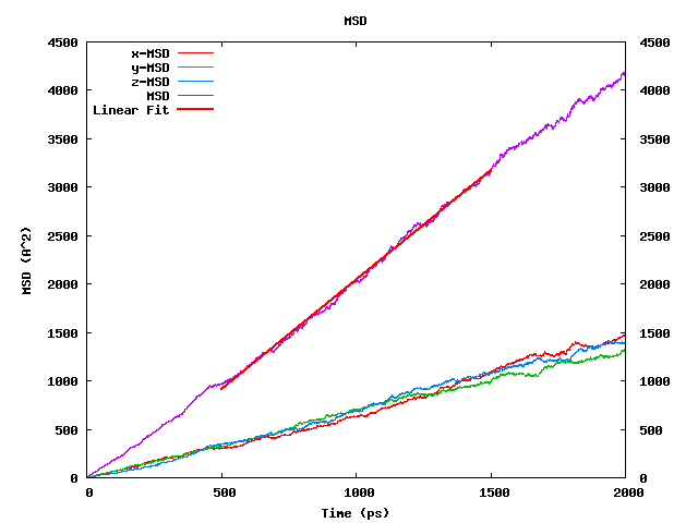
Figure 26.2.4.2 The MedeA Diffusion also module plots MSD values versus time averaged for all diffusing species.
As expected for a homogeneous liquid, the x, y, and z components are equivalent. The straight, red line labeled “Linear fit” indicates the portion of the run used for the actual analysis.
26.2.5. Fitting the computed data
The self-diffusion coefficient depends directly on the slope of the MSD-vs-time plot. For MSD analysis, MedeA selects a central region with 25% of the trajectory on each side, not used for analysis. The reason for this choice is that during the first part of the run, dynamics take place in a ballistic regime, where the MSD is proportional to t², whereas the last part of the MSD plot is affected by the sample averaging scheme requiring data to the “left and right” on the time axis. In a “well -behaved” system, the time evolution of the MSD should be linear in the “middle” region, which is the case in Figure 26.2.4.2.
MedeA summarizes the results of the linear regression fit in the job.out file shown in in Figure 26.2.5.1.
Results for a system of 200 toluene molecules at 328K: Running averages for total energy and temperature during two nanoseconds of NVE simulation.
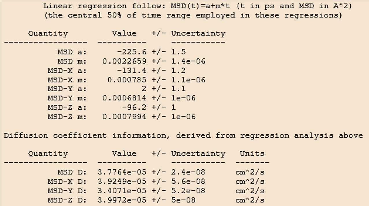
Figure 26.2.5.1 MedeA job.out: Linear regression summary and results for the average diagonal component of the self-diffusion tensor (D=1/3(Dxx + Dyy + Dzz)) and the diagonal components MSD-i D = Dii with i=x,y,z.
The upper table in Figure 26.2.5.1 lists linear regression results for the MSD over time, including the slope m.
The lower table prints the diagonal components of the self-diffusion tensors calculated from the directional MSD values (MSD-i D) and the averaged value (MSD D).
The uncertainties provided in the output correspond to the statistical error of the linear regression fit. While this uncertainty is generally small, the calculated results may vary with the initial configuration, especially when the system contains large or rigid molecules such as oligomers and polymers. Performing several calculations starting from separate fluid configurations will help to estimate the importance of configuration sampling.
26.3. Results
We now discuss results for the self-diffusion coefficient of toluene computed at 328 K, using the calculated data to address the impact of the simulation box size on precision. We then take a look at temperature evolution, comparing computed self-diffusion coefficients for both toluene and acetone with experimental results. Finally, we fit an Arrhenius law to interpolate and extrapolate self-diffusion coefficients to temperatures outside the calculated range.
26.3.1. Finite Size Effects
Figure 26.3.1.1 shows computed self-diffusion coefficients D(N) (blue squares) as a function of the number of molecules N for simulation boxes of varying sizes at constant density. Our earlier calculation for 200 toluene molecules in a 30 Ang3 box corresponds to ~1/N1/3= 0.171 on the x-axis. We note that the computed data is affected by the model size. Assuming linear behavior and extrapolating a linear regression (blue dotted line) to 1/N1/3 ->0, we find the limit of an infinite size model, D∞ = 3.66 x 10⁻⁵ cm²/s.
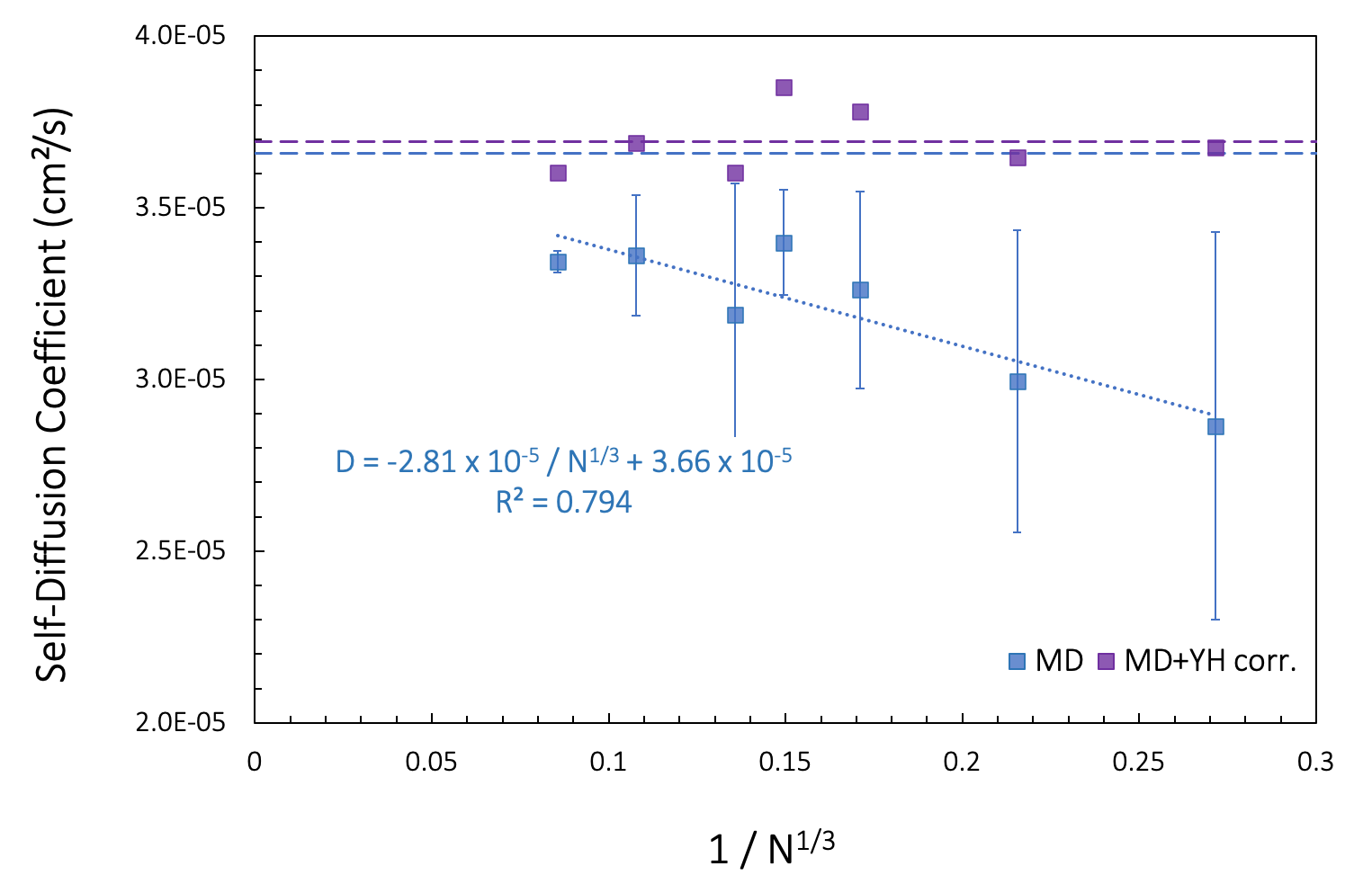
Figure 26.3.1.1 Self-diffusion coefficients calculated for fluid toluene models of different sizes at 328 K. N is the number of molecules in the simulation cell. Blue squares [2] signify computed values. The horizontal blue dashed line is \(D^{\infty}\) obtained from extrapolation of the linear regression to infinite box size (1/N1/3 \(\rightarrow\) 0). Purple squares correspond to adding the Yeh-Hummer correction term, based on the experimental viscosity [12] of 393 \(\mu\)Pa.s. The purple dashed line is D∞ obtained from the averaged of the corrected values.
An alternative method to derive D∞ using a correction term based on the shear viscosity (Figure Figure 26.3.1.1) was proposed by Yeh and Hummer [11] [5].
Yeh and Hummer correlation
where \(k_{B}\) is the Boltzmann constant, \(T\) is the absolute temperature, \(\zeta\) is a dimensionless constant (~2.83), \(\eta\) is the shear viscosity, and \(L\) is the cell length.
We can use their model in two ways:
- If the shear viscosity is available from experiment, literature, or simulation, we can calculate D∞ using just one simulation box size.
- Estimate the fluid viscosity from D(N) values computed at different box sizes via linear regression and D∞.
For our toluene example, the experimental viscosity is 393 \(\mu\)Pa.s at 330 K [10]. Applying the resulting correction term to our computed D(N), we note a slight variation of D∞ (purple squares in Figure 26.3.1.1).
The viscosity, calculated from D(N) and D∞ extracted from the linear regression, is of 243 \(\mu\)Pa.s, somewhat underestimating the recommended experimental value of 393 \(\mu\)Pa.s for T = 330 K.
26.3.2. Temperature dependence of the self-diffusion coefficient
To determine the effect of temperature on the self-diffusion coefficients, we run the diffusion workflow as presented above, but including a loop over temperature from 328 K to 268 K. In Figure 26.3.2.1., we show results for a single fluid configuration with 200 molecules of acetone and toluene and without taking into account the finite size effect.
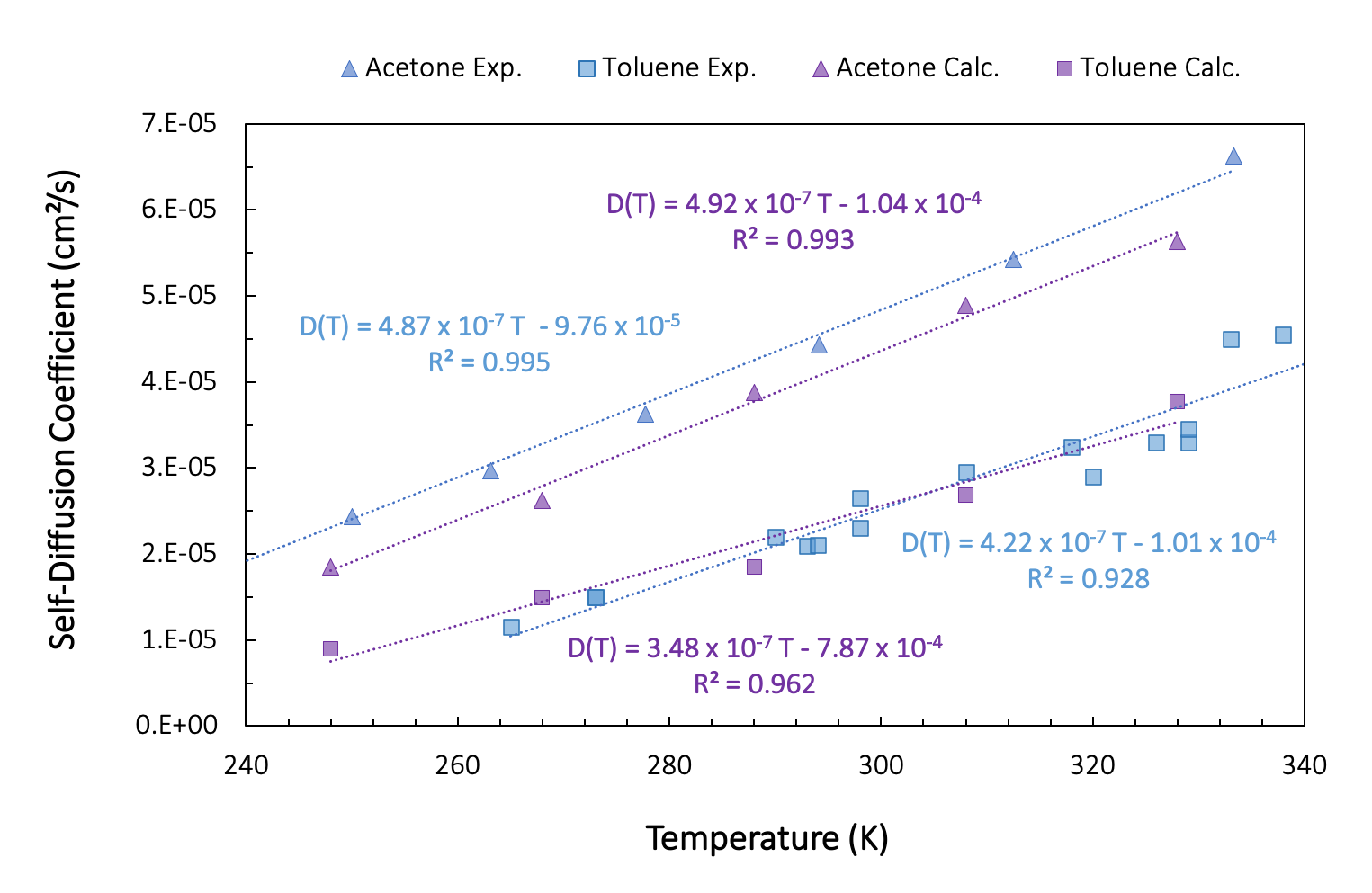
Figure 26.3.2.1 Self-diffusion coefficients for varying temperatures. Purple: Computed, Blue: Experiment.
Despite the small system size, single fluid configuration, and rather short simulation time, the computed self-diffusion coefficients are in relatively good agreement with the experiment.
For toluene, the experimental results are a compilation of experimental data extracted from work by Guevara-Carrion et al. [4]. Our computed values are within the spread of experimental data, whereas for acetone, the calculated values are systematically smaller than the experimental values.
Within a narrow temperature range, we can consider the temperature dependence of the diffusion coefficient as linear. Over a broader range of temperatures, the Arrhenius equation provides a better description. The experimental results provided for acetone in Figure 26.3.1.1 come from such an Arrhenius representation (D0 = 1.34 ± 0.14 x 10⁻³ cm²/s, E = 8.33 ± 0.25 kJ/mole) fitted on 12 experimental data points, and covering a temperature range from 183 to 331 K. The estimated error is approximately 1.93 % [13] .
Figure 26.3.2.1 shows an Arrhenius plot of our computed data for toluene and acetone.
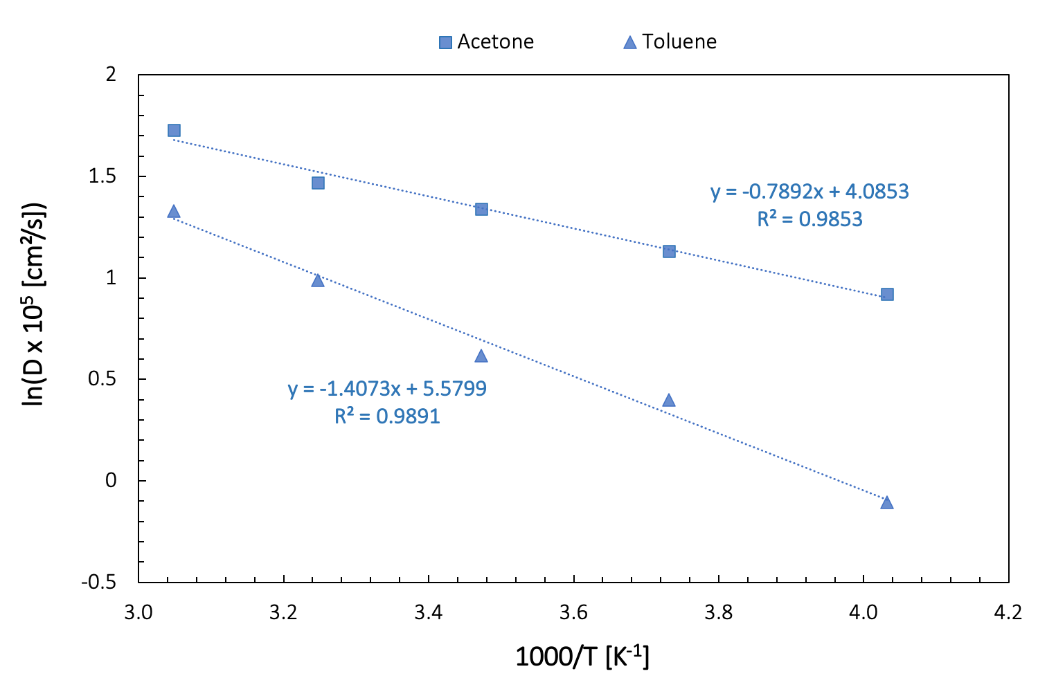
Figure 26.3.2.2 Arrhenius plot of diffusivities of toluene and acetone
| \(D_{0}\) [cm2] | \(E\) [kJ/mol] | |
|---|---|---|
| Acetone | 5.95 x 10⁻⁴ | 6.55 |
| Toluene | 2.65 x 10⁻³ | 11.69 |
The linear fit obtained from our “crude” calculations is not perfect, with R-square values inferior to 0.99. These results can be improved significantly by increasing the simulation length and by performing calculations on several fluid configurations with a somewhat larger number of molecules.
26.3.3. Interpolating
In Figure 26.3.3.1, we show experimental data for the self-diffusion coefficient of acetone at 298 K by Suarez-Iglesias et al. [14], together with our predicted values, obtained both through linear regression and by an Arrhenius plot. Applying the Yeh and Hummer correction term to our linear regression data shifts the self-diffusion coefficient up to 4.9 x 10⁻⁵ cm²/s.
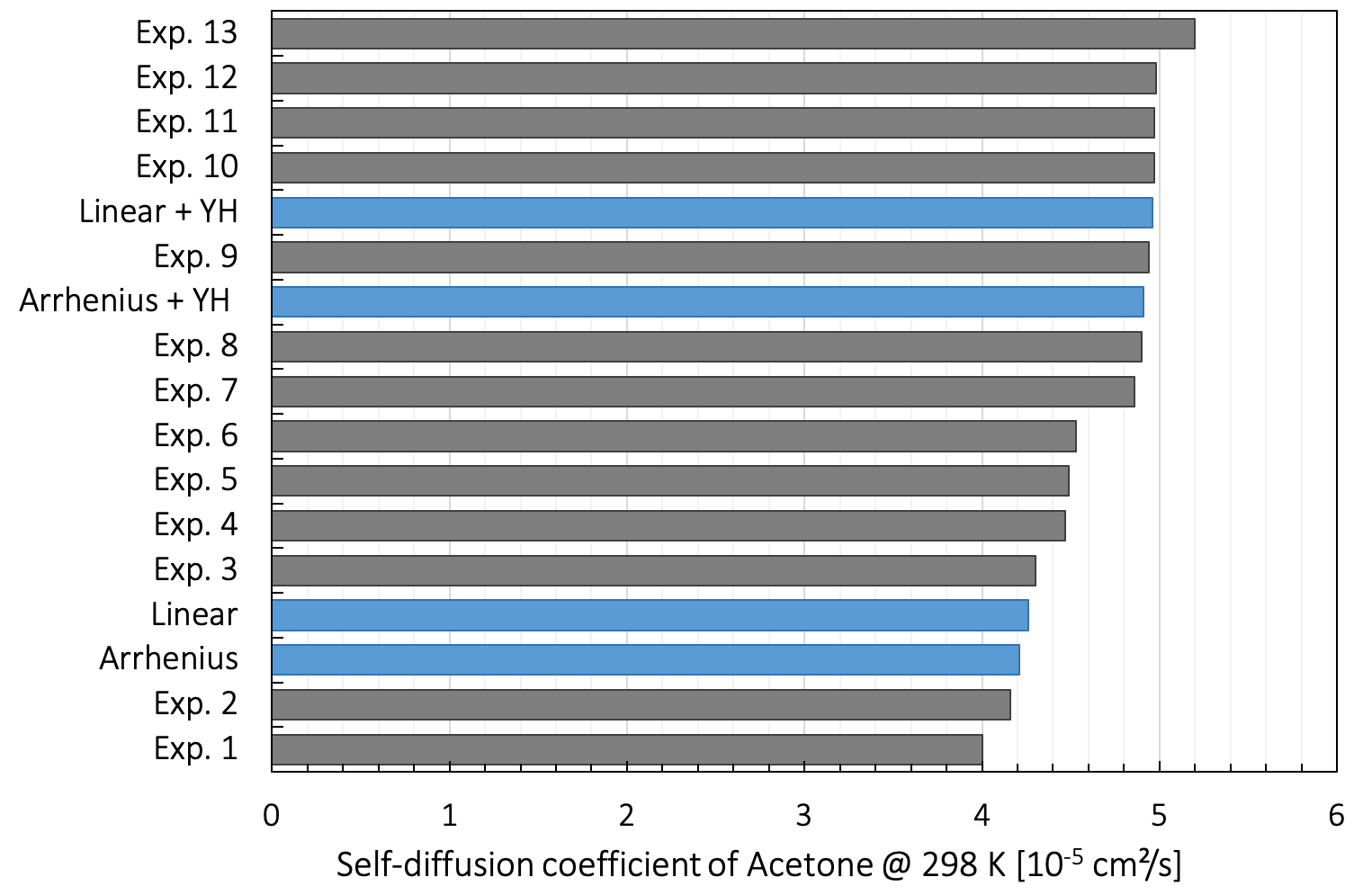
Figure 26.3.3.1 Dispersion of the experimental self-diffusion coefficient of acetone at 298 K in blue measured by different NMR techniques as collected by Suarez-Iglesias, together with our predicted values interpolated using different fits.
The experimental results are obtained using various diffusometry techniques. We name standard pulsed-field gradient NMR, standard pulsed-field gradient NMR combined with magic angle spinning, steady field-gradient NMR, and intravoxel incoherent motion imaging. The predicted values are in the range of the experimental values even though closer to the lower bound than the median value evaluated at 4.6 x 10⁻⁵ cm²/s.
26.3.4. Extrapolating
Extrapolation to higher and lower temperatures also provides a good agreement with experimental data, as presented in Figure 26.3.4.1.
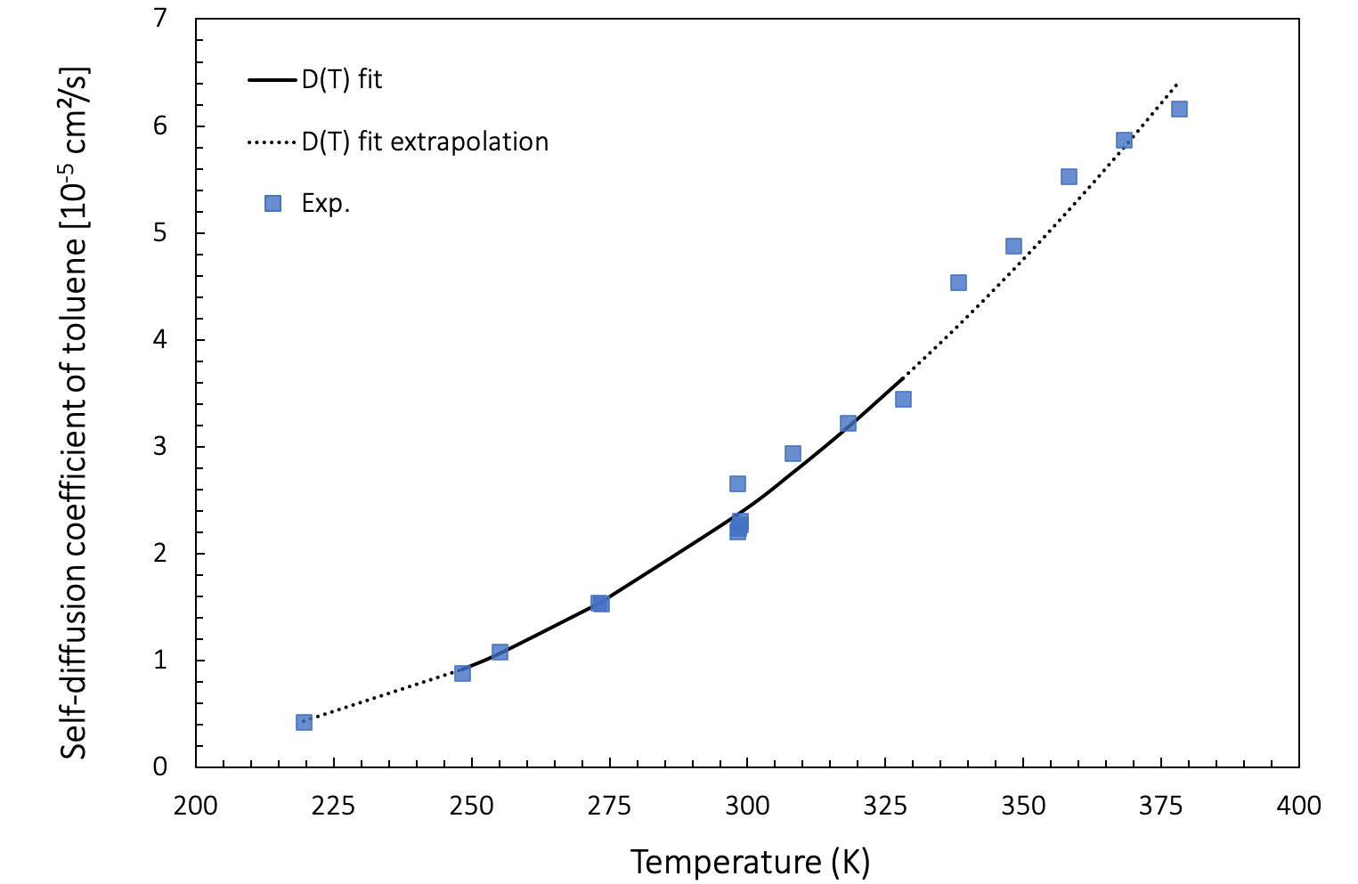
Figure 26.3.4.1 Self-diffusion coefficient as a function of temperature: Arrhenius fit of values computed between 248 K and 328 K (full black line) and extrapolation to lower and higher temperatures (dotted black line), together with experimental results (blue squares).
In a range from 219 K to 298 K, the predicted values for toluene are in good agreement with experiments by Harris [15]. For 298 K - 378 K, our computations also match experimental data obtained by Pickup [16]. The match is good even when extrapolated to lower and higher temperatures
At lower temperatures, diffusion events become increasingly rare. Molecular dynamics simulations aimed at capturing these events need to run for exponentially longer durations times. Therefore, it is often convenient to simulate diffusion at higher temperatures and extrapolate the computed data to lower temperatures using an Arrhenius fit.
26.4. Summary and outlook
Molecular simulations can accurately and with modest computation effort, predict self-diffusion coefficients for pure fluids such as toluene and acetone. Controlling convergence and precision of the necessary molecular dynamics simulations requires understanding the following parameters:
- for convergence to the diffusive regime:
- energy and temperature drift during NVE ensemble dynamics
- the slope of the log-log plot of the global MSD averaged over time
- for precision:
- simulation duration
- averaging over several initial configurations
- error due to the finite size of the simulation box
Self-diffusion coefficients obtained from computations for acetone and toluene at different temperatures compare well with experimental data. Extrapolation to higher and lower temperatures is feasible using an Arrhenius plot. This technique is recommended especially for lower temperatures where molecular dynamics become much slower and hence more time/resource consuming.
We can expand this protocol to obtain the pressure dependence of self-diffusion coefficients for given temperatures.
Addressing mutual diffusion coefficients in predictive models for more complex mixtures requires the input of self-diffusion coefficients for each constituent. Molecular dynamics can thus play a vital role in modeling mass transport phenomena. Further information can be found in the literature [17] [4].
| [1] | MedeA and Materials Design are registered trademarks of Materials Design, Inc. |
| [2] | The error bars are the standard deviations calculated from self-diffusion coefficient obtained for independent configurations with (number of molecules ; number of independent configurations):(50 ; 10)/(100 ; 10)/(200 ; 5) (300 ; 5)/(400 ; 5)/(800 ; 3)/(1600 ; 2) |
| [3] | C. Nieto-Draghi, P. Bonnaud, P. Ungerer “Anisotropic United Atom Model Including the Electrostatic Interactions of Methylbenzenes. II. Transport Properties”, J. Phys. Chem. 111, 15942 (2007)(DOI) |
| [4] | (1, 2, 3) G. Guevara-Carrion, T. Janzen, Y. Mauricio-Munoz-Munoz, J. Vrabec “Mutual diffusion of binary liquid mixtures containing methanol, ethanol, acetone, benzene, cyclohexane, toluene, and carbon tetrachloride”, J. Chem. Phys. 144, 124501 (2016) (DOI) |
| [5] | (1, 2) T.J.P. dos Santos, C.R.A. Abreu, B.A.C. Horta, F.W. Tavares “Self-diffusion coefficients of methane/n-hexane mixtures at high pressures: An evaluation of the finite-size effect and a comparison of force fields”, J. Super. Fluids, 155, 104639 (2020) (DOI) |
| [6] | L.S. Darken, “Diffusion, mobility and their interrelation through free energy in binary metallic systems “, Trans. Am. Inst. Mining. Met. Eng., 175, 184 (1948) (DOI) |
| [7] | J. Li, H. Liu, Y. Hu, “A mutual-diffusion-coefficient model based on local composition”, Fluid Phase Equilib., 187-188, 193 (2001) (DOI) |
| [8] | C. D’Agostino, M.D. Mantle, L.F. Gladden, Mogridge G.D., “Prediction of binary diffusion coefficients in non-ideal mixtures from NMR data: Hexane-nitrobenzene nears its consolute point”, Chem. Eng. Sci., 66, 3898 (2011) (DOI) |
| [9] | S. Plimpton, “Fast Parallel Algorithms for Short-Range Molecular Dynamics,” 1995. |
| [10] | PCFF was developed by the Biosym Potential Energy Functions and Polymer Consortia between 1989 and 2004. Since 2009, PCFF+ has been developed at Materials Design in order to improve the density and cohesive properties of a large number of organic liquids and polymers under ambient conditions. |
| [11] | (1, 2) E.J. Maginn, R.A. Messerly R.A., D.J. Carlson, D.R. Roe, J.R. Elliott “Best practices for computing transport properties 1. Self-Diffusivity and viscosity from equilibrium molecular dynamics”, Living J. Comp. Mol. Sci., 1, 1 (2018) (DOI) |
| [12] | F.J.V. Fernando, C.A.N. de Castro, J.H. Dymond, N.K. Dalaouti, M.J. Assael, A. Nagashima “Standard Reference Data for the Viscosity of Toluene”, J. Phys. Chem. Ref. Data, 35, 1 (2006) (DOI) |
| [13] | H. Ertl and F.A.L. Dullien “Self-diffusion and viscosity of some liquids as function of temperature”, AIChE J., 19, 1215 (1973) (DOI) |
| [14] | O. Suarez-Iglesias, I. Medina, M. de los Angeles Sanz, C. Pizarro, J.L. Bueno “Self-diffusion in molecular fluids and noble gases: Available data”, J. Chem. Eng. Data, 60, 2757 (2015) (DOI) |
| [15] | K.R. Harris, J.J. Alexander, T. Goscinska, R. Malhotra, L.A. Woolf, J.H. Dymond “Temperature and density dependence of the self-diffusion coefficients of liquid n-octane and toluene”, Molecular Physics, 78, (1993) (DOI) |
| [16] | S. Pickup and F.D. Blum, “Self Diffusion of Toluene in Polystyrene Solutions”, Macromolecules, 22, 3961 (1989) (DOI) |
| [17] | X. Liu, S.K. Schnell, J.M. Simon, P. Krüger, D. Bedeaux, S. Kjelstrup, A. Bardow, T.J.H. Vlugt “Diffusion coefficients from molecular dynamics simulations in binary and ternary mixtures”, Intl. J. Thermo., 34, 1169 (2013) (DOI) |
Required Modules
- MedeA Environment including the modules Molecular Builder, LAMMPS, LAMMPS GUI, Flowcharts, Forcefield Bundle and job control (JobServer and TaskServer)
- MedeA Amorphous Materials Builder
- MedeA Diffusion
| download: | pdf |
|---|