29. The \(\alpha\)-\(\beta\)-phase-transition in Ti investigated using a machine-learned interatomic potential
The \(\alpha\)-\(\beta\)-phase transition of Ti is addressed by performing MedeA®[1] LAMMPS classical molecular dynamics simulations, which build upon a machine-learned potential (MLP) trained from MedeA VASP calculations. The efficient creation of a training set, the generation of the MLP using the MedeA MLP Generator, and the application of the MLP are described in detail.
Keywords: Metals, phase stability, phase transitions, machine learning, machine-learned potentials
29.1. Introduction
The phase stability of elemental metals, metallic compounds, and alloys is of great interest [2]. Knowledge of stable phases at ambient conditions, and their transformations into new phases, for example, under varying temperature and/or pressure is vital in many applications. Specific compositions and processing can likewise be of considerable importance. For example, INVAR, an alloy famously composed of precisely 64% Fe and 36% Ni, possesses almost vanishing thermal expansion, understanding the physical basis for such phenomena opens great opportunities for efficiency, innovation, and process improvement. Knowledge of the properties of metals and alloys has benefited tremendously from the introduction of density functional theory (DFT). Such methods explain, e.g., the phase stability of the transition metals and the well known hexagonal close-packed \(\rightarrow\) body-centered cubic \(\rightarrow\) hexagonal close-packed \(\rightarrow\) face-centered cubic crystal structure sequence along the d series. Recent interest has turned to complex metallic systems such as high-entropy alloys demanding larger system calculations..
Despite the incredible increase in computing power seen in the last decades, DFT calculations of large systems are still computationally demanding. In particular, ab initio molecular dynamics simulations of large systems comprising 100,000 or more atoms at long simulation times remain out of reach. As a consequence, phenomena occurring at elevated temperatures, such as temperature-induced phase transitions, can not be well investigated. This severely reduces the applicability of ab initio calculations just when accurate results are needed, restricting their relevance for industrial applications.
For many years the need for large-scale molecular dynamics (MD) simulations was met by the use of classical forcefields. Especially for metals the Embedded Atom Model (EAM) potential by Zhou et al. [3] has proven very useful in a large number of applications. However, being inspired by physical models in terms of bonds and atomic densities, applicability of classical forcefields, e.g., to the study of phase transitions and chemical reactions is limited. In addition, determination of forcefield parameters for new materials requires a lot of expertise and careful fitting.
In the last decade, the restrictions of classical forcefields initiated the development of so-called machine-learned potentials (MLPs). They employ a set of general parametrizable mathematical functions to describe the dependence of the energy, forces, and stress on atomic structure. These parameters are determined from DFT calculations performed on a set of structures, the so-called training set, using machine-learning techniques. Several approaches are used to date including neural-network and regression methods.
The present application note aims to demonstrate the procedure used to generate such MLPs and their capabilities with the example of elemental Ti. As indicated above, Ti as the second element of the 3d series assumes the hexagonal close-packed structure in the \(\alpha\)-phase but undergoes a transition to the body-centered cubic \(\beta\)-phase at about 1156 K. A detailed investigation of this \(\alpha\)-\(\beta\)-phase transition is beyond the capabilities of ab initio calculations. Prior to investigating the transition, the generated MLP is validated with calculations of the elastic properties.
29.2. Calculational Procedure
Generation of an MLP with MedeA’s new Machine-Learned Potential Generator (MLPG) has to be preceded by the creation of a training set including a variety of structures and the execution of DFT calculations for these structures using MedeA VASP. The computational parameters for all these calculations should be identical in order to guarantee consistency of the calculated energies, forces, and stresses.
For the particular case of Ti, the training set comprised more than 1000 structures including the hexagonal close-packed, face-centered cubic, and body-centered cubic structures as well as the \(\omega\)-phase, which is another hexagonal phase found at slightly elevated energies compared to the hexagonal close-packed phase. In addition to these ideal structures, vacancy structures, structures with self-interstitial atoms, and surface structures were considered. Furthermore, NPT MD simulations for a range of temperatures as well as calculations for strained structures were included.
Once the training set calculations have been completed and all data stored in a fitting data set with the help of the MedeA Fitting Data Manager, the MedeA MLPG can be invoked to generate the MLP. For the present purpose, a Spectral Neighbor Analysis Potential (SNAP) has been generated using the FitSNAP code [4], [5], [6]. The resulting MLP is stored in the form of an frc file for use with MedeA LAMMPS.
Energies and forces as obtained from the linear regression underlying the FitSNAP code versus the respective DFT values are displayed in Figure 29.2.1. A very good fit has been achieved with only few outliers, which still are found close to the diagonal.
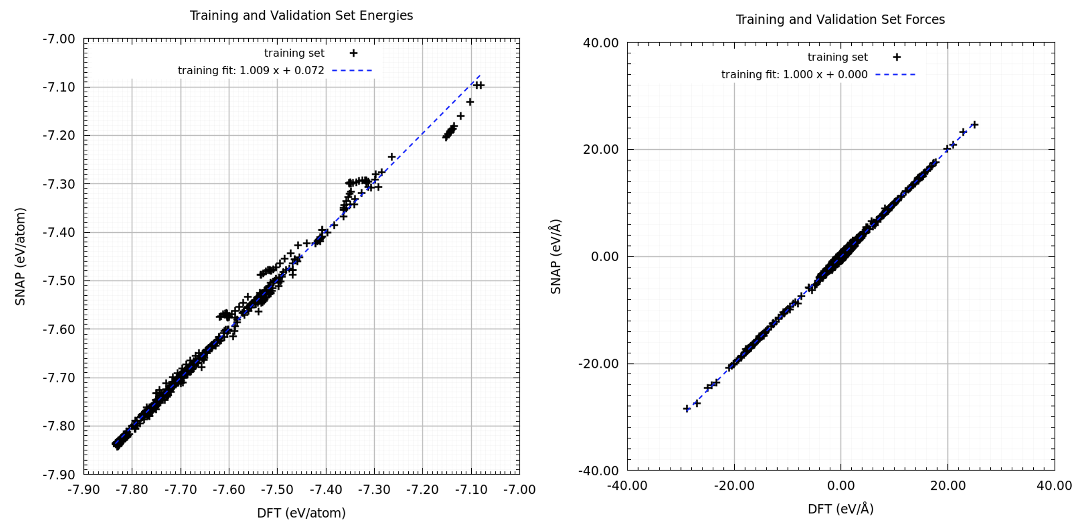
Figure 29.2.1 Energies and forces obtained from the FitSNAP code versus the respective DFT values.
29.3. Validation of the MLP
To validate the generated MLP, lattice parameters of \(\alpha\)-phase and \(\beta\)-phase Ti were calculated from MedeA VASP as well as MedeA LAMMPS using the EAM potential by Zhou et al. [3] and the generated SNAP MLP. The results are given together with experimental data [7] in Figure 29.3.1. Good agreement between the results obtained from the DFT calculations and SNAP MLP is found, while the EAM results agree better with the experimental data. This is related to the fact that the SNAP MLP is constructed from DFT calculations, whereas the construction of the EAM potential takes experimental data into account.
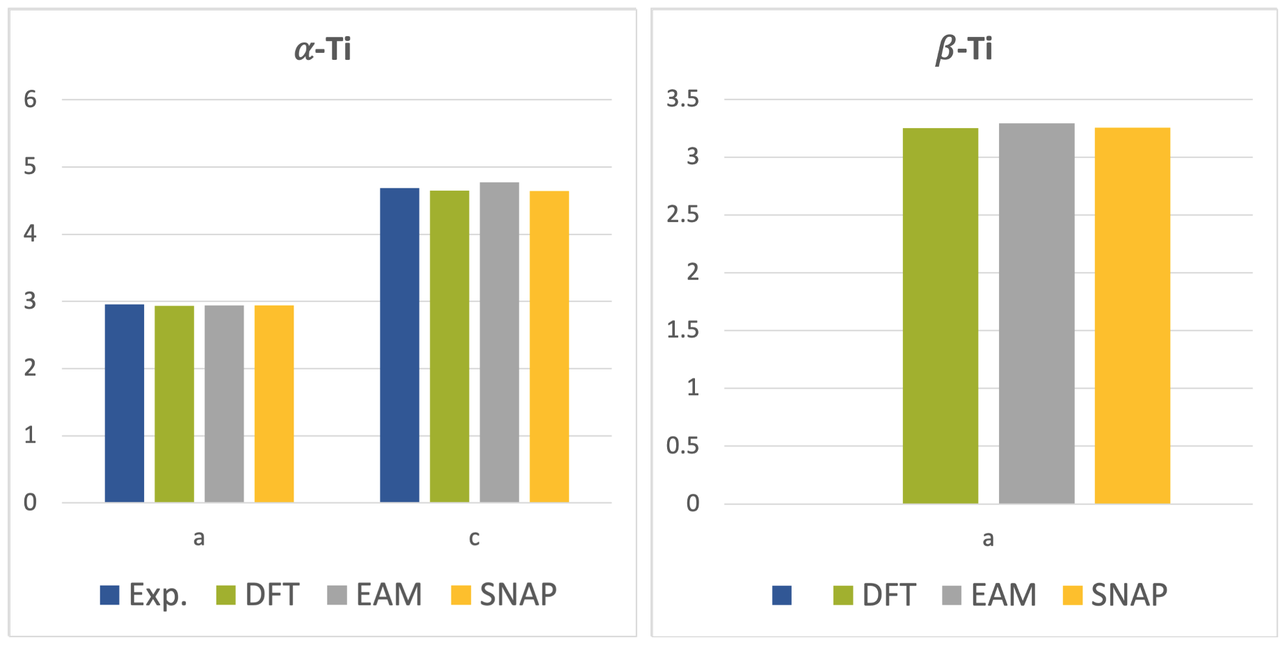
Figure 29.3.1 Lattice parameters of \(\alpha\)-phase and \(\beta\)-phase Ti. All values in \({\mathring{\mathrm{A}}}\).
The situation is different for the elastic coefficients and moduli presented in Figure 29.3.2 and Figure 29.3.3, which show good agreement of the results obtained from MedeA LAMMPS using the SNAP MLP with those from MedeA VASP and also with the experimental data but reveal deviations of the EAM results from some of the experimental data, especially for the \(\beta\)-phase [8], [9].
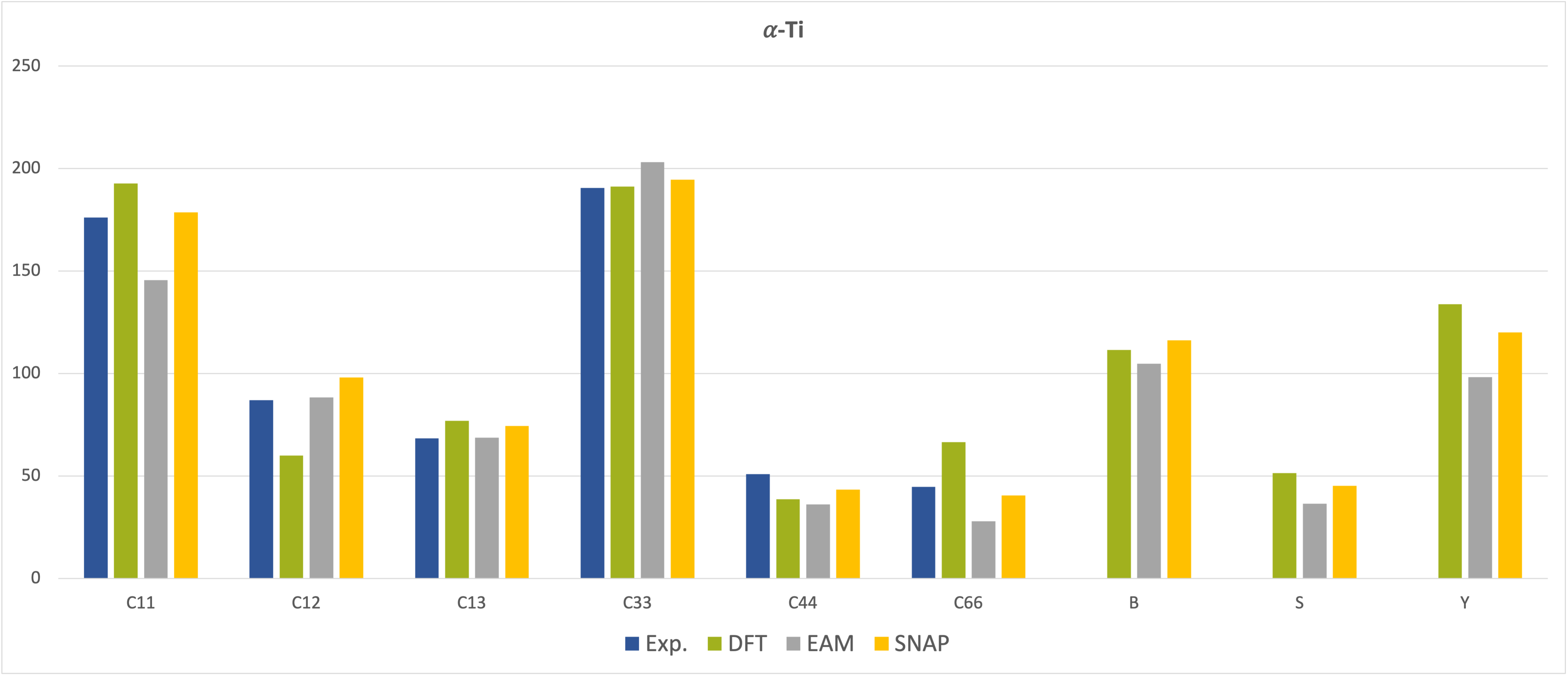
Figure 29.3.2 Elastic constants and moduli of \(\alpha\)-phase Ti. All values in GPa.
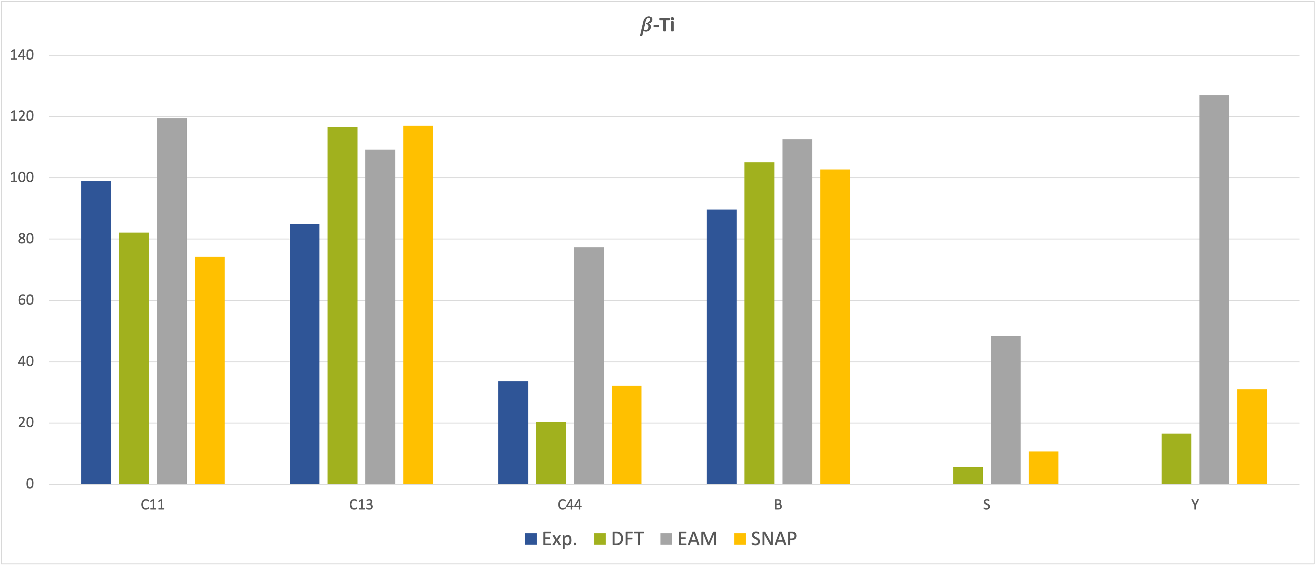
Figure 29.3.3 Elastic constants and moduli of \(\beta\)-phase Ti. All values in GPa.
29.4. The \(\alpha\)-\(\beta\)-phase transition
While the previous results could be obtained from both ab initio and forcefield calculations and thus served to validate the MLP, investigation of the \(\alpha\)-\(\beta\)-phase transition is beyond the capabilities of DFT methods and, hence, MLPs can play out their full potential, namely, their high efficiency paired with the accuracy inherited from DFT.
In order to illustrate the strength of MLPs, the \(\alpha\)-\(\beta\)-phase transition was investigated by performing molecular dynamics simulations at a variety of temperatures between 300 K and 2200 K using MedeA LAMMPS with the generated SNAP MLP. At each temperature, supercell structures were equilibrated for 20 ps at a timestep of 1 fs. In particular, on heating and cooling, simulations started at 300 K and 2200 K with supercells of the hcp and bcc structures comprising 180 and 192 atoms, respectively. The energies of the equilibrated structures at each temperature are displayed in Figure 29.4.1.
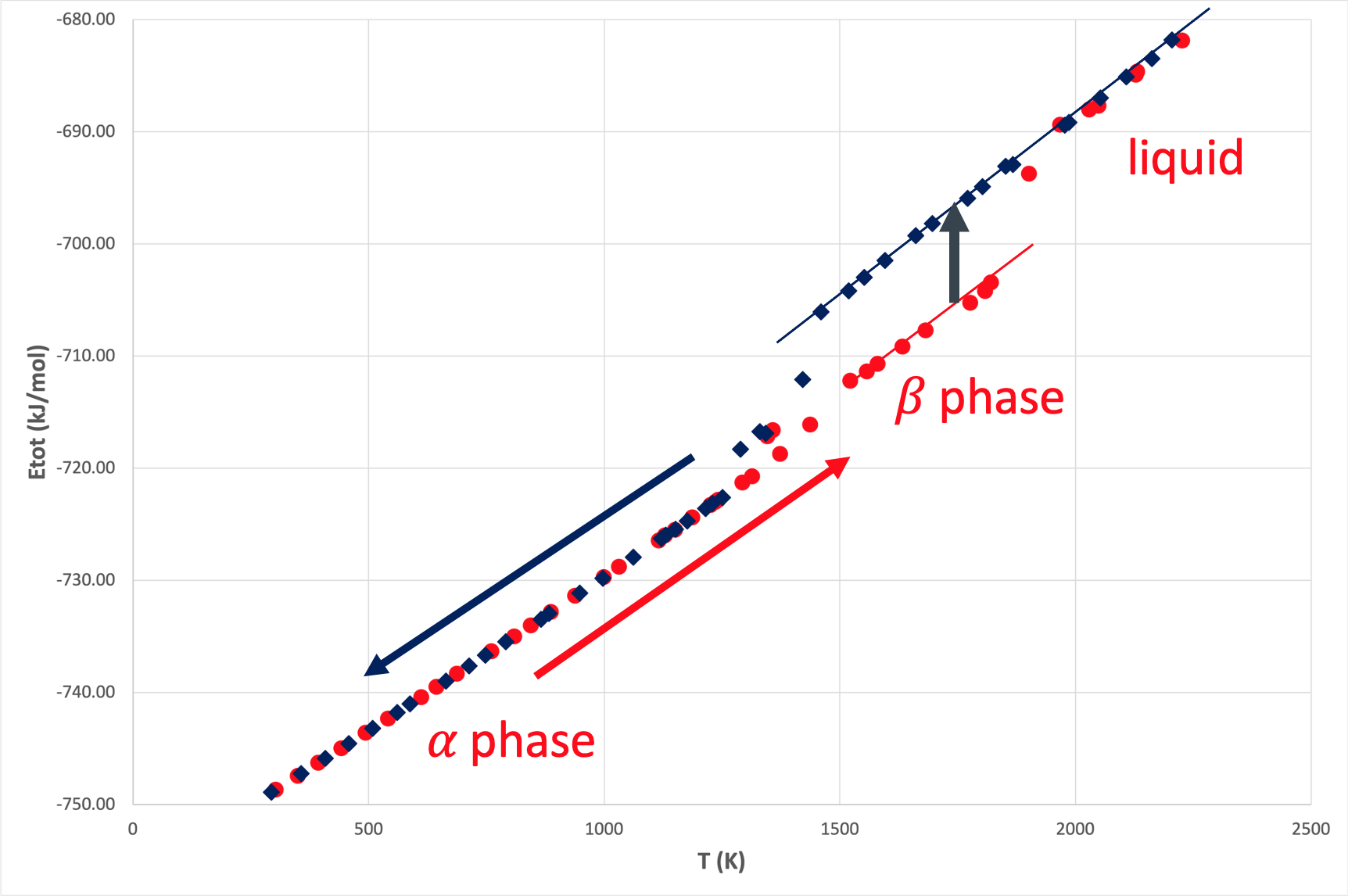
Figure 29.4.1 Energies of equilibrated supercell structures as a function of temperature on heating (red) and cooling (blue).
On heating, two different phase transitions are observed. At about 1300 K, the \(\alpha\)-structure starts to transform into the \(\beta\)-structure and between 1800 K and 2000 K melting sets in. These temperatures compare rather well with the experimentally observed transition temperatures of 1156 K and 1946 K, respectively.
While the computed specific heats vary between 28-30 J/(mol K) in good agreement with the measured data of 25-37 J/(mol K) [10], [11], the calculated latent heat of the \(\alpha\)-\(\beta\)-phase transition and the calculated heat of fusion are 2.7 kJ/mol and 10.4 kJ/mol, respectively, hence, slightly below the experimental values of 3.6-4.3 kJ/mol [11], [12] and 13 kJ/mol [13].
Hence, the MLP generated here accurately describes the \(\alpha\)-\(\beta\)-phase transition and reproduces key thermodynamic data. Given the moderate size of the training set and the relatively small size of the supercell structures used in these illustrative calculations, these results demonstrate the efficiency and utility of MLPs. This success is underlined by the fact that additional calculations using the EAM potential by Zhou et al., while being able to describe the melting process, are unable to reproduce the \(\alpha\)-\(\beta\)-phase transition.
Additional analysis of the structural changes occurring at the transitions has been undertaken. Here models equilibrated at 1700 K and 2200 K were investigated in using calculated pair correlation functions at various temperatures. These results are displayed in Figure 29.4.2.
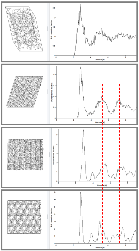
Figure 29.4.2 Pair correlation functions of equilibrated supercell structures taken at different temperatures. From top to bottom: 2200 K (heating), 1700 K (heating), 300 K (bcc), 300 K (hcp).
Specifically, the calculated pair correlation function of the structure observed at 1700 K on heating revealed a clear resemblance with that of the \(\beta\)-phase calculated at 300 K and distinct deviations from that of the \(\alpha\)-phase calculated at the same temperature. In addition, the pair correlation function of the structure obtained at 2200 K showed strong signatures of the liquid phase. Thus, like the energies, the equilibrated structures provide clear indications of the phase transitions.
29.5. Conclusion
This application note illustrates the investigation of the \(\alpha\)-\(\beta\)-phase transition of Ti using MedeA LAMMPS with a machine-learned potential (MLP) as generated by the MedeA MLP Generator. Key quantities such as the transition temperature, melting point, latent heats, and specific heat capacities in addition to elastic properties are very well described by the calculations, demonstrating the broad applicability of tailor-made MLPs and their accuracy and efficiency in the investigation of long length and time scale effects at finite temperatures. All of the steps described here, the creation of the training set, the generation of the MLP itself, and the use of the MLP in computing physical properties were conducted in the MedeA materials simulation and productivity environment.
MedeA modules used in this application
- MedeA Environment
- MedeA VASP
- MedeA MLPG
- MedeA LAMMPS
- MedeA MT
- MedeA Phonon
| [1] | MedeA and Materials Design are registered trademarks of Materials Design, Inc. |
| [2] | J. Kübler and V. Eyert, “Electronic structure calculations”, in: “Electronic and Magnetic Properties of Metals and Ceramics”, ed. K. H. J. Buschow (VCH Verlagsgesellschaft, Weinheim 1992), pp. 1-145; Volume 3A of “Materials Science and Technology - A Comprehensive Treatment”, ed. R. W. Cahn, P. Haasen, and E. J. Kramer (VCH Verlagsgesellschaft, Weinheim 1991-1996). (DOI) |
| [3] | (1, 2) X. W. Zhou, R. A. Johnson, and H. N. G. Wadley, “Misfit-energy-increasing dislocations in vapor-deposited CoFe/NiFe multilayers”, Phys. Rev. B 69, 144113 (2004) (DOI) |
| [4] | A. P. Thompson, L. P. Swiler, C. R. Trott, S. M. Foiles, and G. J. Tucker, “Spectral neighbor analysis method for automated generation of quantum-accurate interatomic potentials”, J. Comp. Phys. 285, 316 (2015) (DOI) |
| [5] | M. A. Wood and A. P. Thompson, “Extending the accuracy of the SNAP interatomic potential form”, J. Chem. Phys. 148, 241721 (2018) (DOI) |
| [6] | M. A. Cusentino, M. A. Wood, and A. P. Thompson, “Explicit Multielement Extension of the Spectral Neighbor Analysis Potential for Chemically Complex Systems”, J. Phys. Chem. A 124, 5456 (2020) (DOI) |
| [7] | R. M. Wood, “The Lattice Constants of High Purity Alpha Titanium”, Proc. Phys. Soc. 80, 783 (1962) |
| [8] | E. S. Fischer and C. J. Renken, “Single-Crystal Elastic Moduli and the hcp –> bcc Transformation in Ti, Zr, and Hf”, Phys. Rev. 135, A482 (1964) (DOI) |
| [9] | E. S. Fischer and D. Dever, “The Single Crystal Elastic Moduli of Beta-Titanium and Titanium-Chromium Alloys”, in: “The Science, Technology and Application of Titanium”, R. I. Jaffee and N. E. Promisel (eds.), (Pergamon Press, New York, NY, 1970), pp. 373–381. |
| [10] | E. Kaschnitz and P. Reiter, “Heat capacity of titanium in the temperature range 1500 to 1900 K measured by a millisecond pulse-heating technique”, J. Therm. Anal. Calorim. 64, 351 (2001) (DOI) |
| [11] | (1, 2) M. Behara, S. Raju, B. Jeyaganesh, R. Mythili, and S. Saroja, “A Study on Thermal Properties and \(\alpha\)(hcp) –> \(\beta\)(bcc) Phase Transformation Energetics in Ti-5mass% Ta-1.8mass% Nb Alloy Using Inverse Drop Calorimetry” Int. J. Thermophys. 31, 2246 (2010) (DOI) |
| [12] | E. Kaschnitz and P. Reiter, “Enthalpy and temperature of the titanium alpha-beta phase transformation”, Int. J. Thermophys. 23, 1339 (2002) (DOI) |
| [13] | J. L. McClure and A. Cezairliyan, “Measurement of the Heat of Fusion of Titanium and a Titanium Alloy (90Ti-6Al-4V) by a Microsecond-Resolution Transient Technique”, Int. J. Thermophys. 13, 75 (1992) (DOI) |
| download: | pdf |
|---|